Slit Interference (Mathematical Explanation With Complex Numbers)

Monday, December 10, 2018

Slit Interference (Mathematical Explanation With Complex Numbers)

Slit Interference

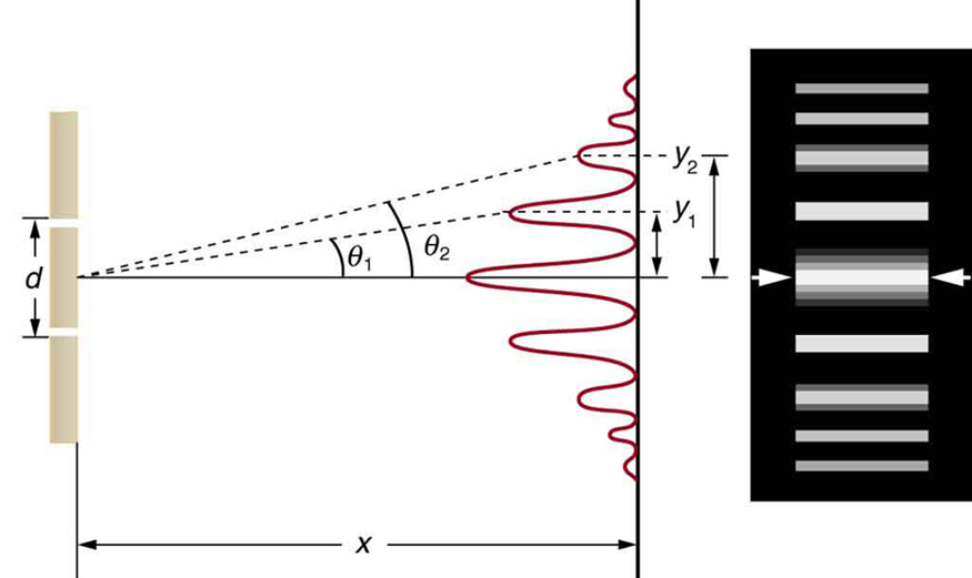
If we have one slit, we take a beam of particles described by a wave function ψ(x)

The simplest wave function would be to have ψ(x) = e^ipx/ħ (where p is the particle's momentum). It passes through the hole and the probability wave spreads out. If we look over a small part of the screen we can model the wave as e^ipy/ħ where the screen is the y axis. The probability of finding the particle at a different y is uniform. This is because if we do e^ipx/ħ x e^-ipx/ħ (its complex conjugate) we get 1. The magnitude of is e^ipx/ħis constant.

If we add a second slit, we get a new wave. It will add to the first wave that we have. This is strange because we are adding states which we would never do in classical physics. You would never think to add a head state of a coin to a tail state to get some sort of superposition of the two.

The second wave will be slightly different to the first because they are at different heights and so we will say it can be described on the screen as e^iqy/ħ. Either one of the waves individually has a magnitude equal to 1 and so we would have a uniform probability distribution. But when we open both slits, the probability distribution is no longer uniform.

Hole 1 |ψ₁>
Hole 2 |ψ₂>
Both holes |ψ₁> + |ψ₂>

The probability of finding different y when both holes are open is given by |ψ₁> + |ψ₂> x its complex complex conjugate.

(e^ipy/ħ + e^iqy/ħ)(e^-ipy/ħ + e^-iqy/ħ)
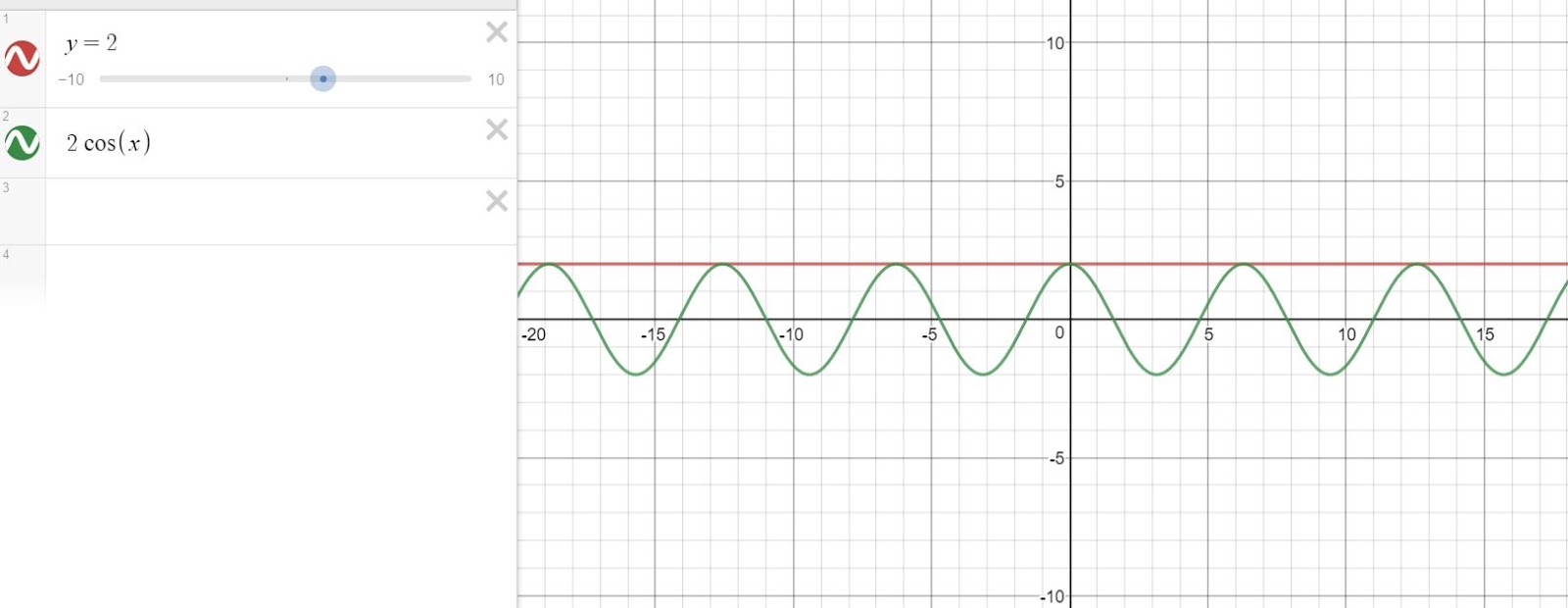
= 2 + e^{i(p - q)y/ħ}+ e^{i(q -p)y/ħ}. (e^ix + e^-ix = 2cos(x))

= 2 + 2cos(p(y-q)/ħ)

= 2(1 + cos(p(y-q)/ħ)

And so the probability went from uniform, when we had one slit, to oscillating, when we have two slits open. The probability has a constant part and an oscillating cos wave

The top graph shows the two parts of the probability separately (its oscillating part and its constant part). The bottom graph combines them to show how the probability of finding a particle changes as we move along the screen.

The key to this was the complex numbers. It turns out that when we had one hole, the particles had an oscillating imaginary part and a uniform real part. The imaginary part has on effect when looking at one slit but when the second slit is opened, you get weird cross-terms from the quadratic which leads to an oscillating probability. I also think it is pretty cool to see that imaginary numbers actually have real life application.

Thanks for reading. If you enjoyed this post or any of my others, follow and subscribe to my blog. Feel free to discuss anything related to this post or ask questions in the comments below.